Aberration Transfer Functions

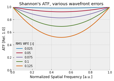
One may find reference on the internet to an “Aberration Transfer Function” introduced by Shannon used to model the MTF of an aberrated imaging system as:

\begin{align*} DTF(\nu) &= \frac{2}{\pi}\left[\arccos{\nu} - \nu \sqrt{1 - \nu^2}\right] \\ ATF(\nu) &= 1 - \left(\frac{W_\text{rms}}{0.18}\right)^2\left(1 - 4(\nu - 0.5)^2\right) \\ MTF(\nu) &= DTF(\nu) \times ATF(\nu) \end{align*}

where \(DTF\) is the diffraction-limited MTF, \(ATF\) is the “Aberration Transfer Function,” \(MTF\) is the modulation transfer function, and \(W_\text{rms}\) is the RMS wavefront error.

In this example, we will show that this treatment should not be used if accuracy is desired from a model. The example should also highlight the terse nature of examples such as this when calculated using prysm.

We begin by importing some classes and functions from the library, and defining the ATF function as Shannon describes it:

import numpy as np

from prysm.otf import diffraction_limited_mtf
from prysm import FringeZernike, PSF, MTF

from matplotlib import pyplot as plt

def shannon_atf(nu, Wrms):
    return 1 - ((Wrms / 0.18) ** 2 * (1 - 4 * (nu - 0.5) ** 2 ))

%matplotlib inline
plt.style.use('bmh')

Wrms_vals = [0.025, 0.05, 0.075, 0.1, 0.125]
nu = np.linspace(0, 1, 100)
atf_curves = []
for Wrms in Wrms_vals:
    atf_curves.append(shannon_atf(nu=nu, Wrms=Wrms))

fig, ax = plt.subplots()
for (curve, label) in zip(atf_curves, Wrms_vals):
    ax.plot(nu, curve, label=label)

ax.legend(title=r'RMS WFE [$\lambda$]')
ax.set(xlim=(0,1), xlabel='Normalized Spatial Frequency [a.u.]',
       ylim=(0,1), ylabel='ATF [Rel. 1.0]',
       title="Shannon's ATF, various wavefront errors");

Now we’ll pick a few different Zernike modes and show the numerically derived version, generated by calculating the MTF numerically and dividing by the diffraction limited MTF for a circular aperture, given above as \(DTF\). The accuracy of prysm’s MTF calculations is sufficiently high that we can ignore that as a reason for the discrepancy. The accuracy of prysm’s MTF calculations is that we can ignore that as a reason for any discrepancy.

# only 20 lines of code, half of which is looping or plotting!
def render_atf_curves_zernike_mode(mode_index, Wrms_vals):
    kwarg = {}

    real_mtfs = []
    for Wrms in Wrms_vals:
        kwarg[f'Z{mode_index}'] = Wrms
        pupil = FringeZernike(**kwarg, norm=True, z_unit='waves')  # waves is the default, not really needed
        psf = PSF.from_pupil(pupil, efl=2)  # normalized frequency makes this choice arbitrary
        mtf = MTF.from_psf(psf)

        u, mtf_ = mtf.slices().x
        real_mtfs.append(mtf_)

    cutoff = 1 / (psf.wavelength * psf.fno) * 1e3 # 1e3 is cy/um => cy/mm
    normalized_frequencies = u / cutoff
    diffraction_limit = diffraction_limited_mtf(psf.fno, psf.wavelength, frequencies=u)

    # don't plot quite all of the curve, division by almost zero is a problem at the end
    fig, ax = plt.subplots()
    for (curve, label) in zip(real_mtfs, Wrms_vals):
        atf = curve / diffraction_limit
        ax.plot(normalized_frequencies[:-5], atf[:-5], label=label)

    ax.legend(title=f'RMS WFE [$\lambda$]')
    ax.set(xlim=(0,1), xlabel='Normalized Spatial Frequency',
           ylim=(0,1), ylabel='ATF',
           title=f'Numerically derived ATF for Fringe Zernike term Z{mode_index}')

    return fig, ax

# Z4 = defocus, the lowest-order Zernike error to affect imaging (and MTF)
render_atf_curves_zernike_mode(4, Wrms_vals)

(<Figure size 432x288 with 1 Axes>,
 <AxesSubplot:title={'center':'Numerically derived ATF for Fringe Zernike term Z4'}, xlabel='Normalized Spatial Frequency', ylabel='ATF'>)

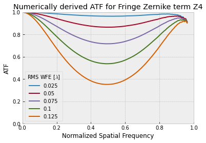
The curve looks broadly similar, but the belly reaches down quite a bit further. What about higher order terms?

# Z9 = "zernike primary spherical" -- low-order spherical aberration
render_atf_curves_zernike_mode(9, Wrms_vals)

(<Figure size 432x288 with 1 Axes>,
 <AxesSubplot:title={'center':'Numerically derived ATF for Fringe Zernike term Z9'}, xlabel='Normalized Spatial Frequency', ylabel='ATF'>)

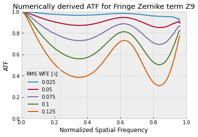
We can see that for low order spherical aberration, the curves look very different. What if we had a higher order variant?

# Z 25 = "zernike tertiary spherical" -- 8th order spherical aberration, in Hopkins' wave aberration expansion
render_atf_curves_zernike_mode(25, Wrms_vals)

(<Figure size 432x288 with 1 Axes>,
 <AxesSubplot:title={'center':'Numerically derived ATF for Fringe Zernike term Z25'}, xlabel='Normalized Spatial Frequency', ylabel='ATF'>)

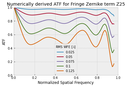
Even worse. These are lots of squiggly lines, what if we directly compare a real ATF for a reasonable wavefront vs Shannon’s ATF equation?

# most of this code is just copy pasted from above
pupil = FringeZernike(Z9=0.1, norm=True, z_unit='waves')  # waves is the default, not really needed
psf = PSF.from_pupil(pupil, efl=2)  # normalized frequency makes this choice arbitrary
mtf = MTF.from_psf(psf)

u, mtf_ = mtf.slices().x

diffraction_limit = diffraction_limited_mtf(psf.fno, psf.wavelength, frequencies=u)

real_atf = mtf_ / diffraction_limit
unormalized = u / (1 / (psf.wavelength * psf.fno) * 1e3)

fig, ax = plt.subplots()

ax.plot(nu, shannon_atf(nu, 0.1), label="Shannon's eq.")
ax.plot(unormalized[:-5], real_atf[:-5], label='Numerical Solution')

ax.legend(title='Method')
ax.set(xlim=(0,1), xlabel='Normalized Spatial Frequency',
       ylim=(0,1), ylabel='ATF',
       title=r'Z9, RMS WFE = 0.1 $\lambda$');

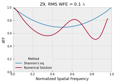
Not a good match. What if we look at the peak error in Shannon’s equation as a function of Zernike index and RMS WFE corresponding to the Marechal critera?

def render_atf_peakerror_vs_zernike(max_zernike=36, rms_wfe= 1 / 14): # 1 / 14 is the Marechal criteria
    # a lot of this code is similar to the earlier function
    peak_errors = []

    # calculate one pilot case to get the metadata for the diffraction limited MTF.  This is a performance optimization
    pupil = FringeZernike()
    psf = PSF.from_pupil(pupil, efl=2)
    mtf = MTF.from_psf(psf)
    u, t = mtf.slices().x

    diffraction_limit = diffraction_limited_mtf(psf.fno, psf.wavelength, frequencies=u)
    cutoff = 1 / (psf.wavelength * psf.fno) * 1e3
    normalized_frequencies = u / cutoff

    shannon = shannon_atf(normalized_frequencies, rms_wfe)

    idxs = list(range(max_zernike+1))
    for i in idxs:
        kwarg = {}
        kwarg[f'Z{i+1}'] = rms_wfe
        pupil = FringeZernike(**kwarg, norm=True, z_unit='waves')  # waves is the default, not really needed
        psf = PSF.from_pupil(pupil, efl=2)  # normalized frequency makes this choice arbitrary
        mtf = MTF.from_psf(psf)

        cutoff = 1 / (psf.wavelength * psf.fno) * 1e3 # 1e3 is cy/um => cy/mm
        u, mtf_ = mtf.slices().x

        atf = mtf_ / diffraction_limit
        difference = abs(shannon[:-10] - atf[:-10])  # erode a little more of the end here for high order cases
        peak_errors.append(difference.max())

    fig, ax = plt.subplots()
    ax.plot(idxs, peak_errors)
    ax.set(xlim=(0,max_zernike), xlabel="Wavefront's Zernike index",
           ylim=(0,1), ylabel="Peak error of Shannon's ATF equation",
           title=f'RMS WFE = {rms_wfe:.3f}' + r'$\lambda$')

    return fig, ax

render_atf_peakerror_vs_zernike(36, rms_wfe=1 / 14)

(<Figure size 432x288 with 1 Axes>,
 <AxesSubplot:title={'center':'RMS WFE = 0.071$\\lambda$'}, xlabel="Wavefront's Zernike index", ylabel="Peak error of Shannon's ATF equation">)

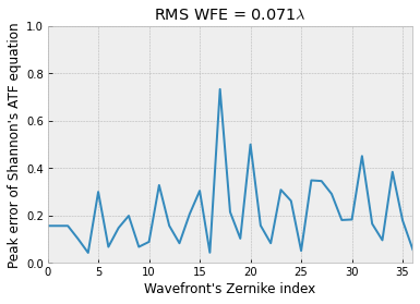
For a wavefront at the Marechal criteria, the error can be as high as 0.7. Since MTF must be within the range [0, 1], this means the error is at least 70%. What if we had a tenth wave RMS?

render_atf_peakerror_vs_zernike(36, rms_wfe=1 / 10)

(<Figure size 432x288 with 1 Axes>,
 <AxesSubplot:title={'center':'RMS WFE = 0.100$\\lambda$'}, xlabel="Wavefront's Zernike index", ylabel="Peak error of Shannon's ATF equation">)

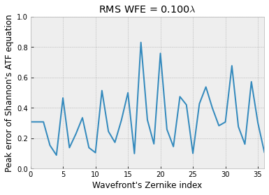
Now the absolute error can be as high as 0.9, again at least 90% due to the normalization of MTF.

Since these errors are so large, we can conclude that Shannon’s ATF function should not be used if accuracy is desired.